42 how to show data labels in excel

Add or remove data labels in a chart - support.microsoft.com Click Label Options and under Label Contains, select the Values From Cells checkbox. When the Data Label Range dialog box appears, go back to the spreadsheet and select the range for which you want the cell values to display as data labels. When you do that, the selected range will appear in the Data Label Range dialog box. Then click OK. Suppressing Data Labels in Excel if #N/A Value - Stack Overflow I had this problem as well and found the easiest solution is to duplicate the chart data fields add those as new series to the chart data change the series chart type for the new fields to a line chart with no line and no marker show the data labels only for those new fields. (column charts will show #N/A, line charts do not). Share

How to Use Cell Values for Excel Chart Labels - How-To Geek Mar 12, 2020 · Make your chart labels in Microsoft Excel dynamic by linking them to cell values. When the data changes, the chart labels automatically update. In this article, we explore how to make both your chart title and the chart data labels dynamic. We have the sample data below with product sales and the difference in last month’s sales.

How to show data labels in excel

Excel, giving data labels to only the top/bottom X% values 1) Create a data set next to your original series column with only the values you want labels for (again, this can be formula driven to only select the top / bottom n values). See column D below. 2) Add this data series to the chart and show the data labels. 3) Set the line color to No Line, so that it does not appear! Prevent Overlapping Data Labels in Excel Charts - Peltier Tech May 24, 2021 · Overlapping Data Labels. Data labels are terribly tedious to apply to slope charts, since these labels have to be positioned to the left of the first point and to the right of the last point of each series. This means the labels have to be tediously selected one by one, even to apply “standard” alignments. How To Create Labels In Excel - inmocasa.info Make Row Labels In Excel 2007 Freeze For Easier Reading from . Starting document near the bottom. Click a data label one time to select all data labels in a data series or two times to select just one data label that you want to delete, and then press delete. Click finish & merge in the finish group on the mailings tab.

How to show data labels in excel. Change the format of data labels in a chart To get there, after adding your data labels, select the data label to format, and then click Chart Elements > Data Labels > More Options. To go to the appropriate area, click one of the four icons ( Fill & Line , Effects , Size & Properties ( Layout & Properties in Outlook or Word), or Label Options ) shown here. How to Add Labels to Show Totals in Stacked Column Charts in Excel Press the Ok button to close the Change Chart Type dialog box. The chart should look like this: 8. In the chart, right-click the "Total" series and then, on the shortcut menu, select Add Data Labels. 9. Next, select the labels and then, in the Format Data Labels pane, under Label Options, set the Label Position to Above. 10. How to add Data Label to Waterfall chart - Excel Help Forum 1. Manually edit the text of the labels. 2. Select each label (two single clicks, one selects the series of labels, the second selects the individual label). Don't click so much as the cursor starts blinking in the label. Click in the formula bar, type an = sign, then click on the cell that contains the label. 3. How To Create Labels In Excel - kimchaurestaurant.com How To Create Labels In Excel. The mail merge feature will. Make a column for each element you want to include on the labels. The next time you open the document, word will ask you whether you want to merge the information from the excel data file. Click finish & merge in the finish group on the mailings tab.

how to add data labels into Excel graphs - storytelling with data You can download the corresponding Excel file to follow along with these steps: Right-click on a point and choose Add Data Label. You can choose any point to add a label—I'm strategically choosing the endpoint because that's where a label would best align with my design. Excel defaults to labeling the numeric value, as shown below. Hiding data labels for some, not all values in a series Here's a good challenge for you. I can't figure it out, and I believe it's a limitation of Excel. I have a bar graph with several data series. I know how to show the data labels for every data point in a given series. But I'm looking to show the data label for only some data points in a given series -- i.e. non-zero valued data points. Find, label and highlight a certain data point in Excel scatter graph Select the Data Labels box and choose where to position the label. By default, Excel shows one numeric value for the label, y value in our case. To display both x and y values, right-click the label, click Format Data Labels…, select the X Value and Y value boxes, and set the Separator of your choosing: Label the data point by name How to show data label in "percentage" instead of - Microsoft Community Select Format Data Labels Select Number in the left column Select Percentage in the popup options In the Format code field set the number of decimal places required and click Add. (Or if the table data in in percentage format then you can select Link to source.) Click OK Regards, OssieMac Report abuse 8 people found this reply helpful ·

Add a DATA LABEL to ONE POINT on a chart in Excel Click on the chart line to add the data point to. All the data points will be highlighted. Click again on the single point that you want to add a data label to. Right-click and select ' Add data label ' This is the key step! Right-click again on the data point itself (not the label) and select ' Format data label '. How to Make a Pie Chart in Excel & Add Rich Data Labels to ... - ExcelDemy 7) With the data point still selected, go to Chart Tools>Format>Shape Styles and click on the drop-down arrow next to Shape Effects and select Shadow and choose Inner Shadow>Inside Diagonal Top Left. 8) With the one data point still selected, right-click this data point, and select Add Data Label>Add Data Callout as shown below. Format Data Labels in Excel- Instructions - TeachUcomp, Inc. To do this, click the "Format" tab within the "Chart Tools" contextual tab in the Ribbon. Then select the data labels to format from the "Chart Elements" drop-down in the "Current Selection" button group. Then click the "Format Selection" button that appears below the drop-down menu in the same area. Adding Data Labels to the Inside Ring of a Sunburst Chart : r/excel Once your problem is solved, reply to the answer (s) saying Solution Verified to close the thread. Follow the submission rules -- particularly 1 and 2. To fix the body, click edit. To fix your title, delete and re-post. Include your Excel version and all other relevant information. Failing to follow these steps may result in your post being ...

Pie Chart - PK: An Excel Expert

Create Dynamic Chart Data Labels with Slicers - Excel Campus Feb 09, 2016 · Step 3: Use the TEXT Function to Format the Labels. Typically a chart will display data labels based on the underlying source data for the chart. In Excel 2013 a new feature called “Value from Cells” was introduced. This feature allows us to specify the a range that we want to use for the labels.

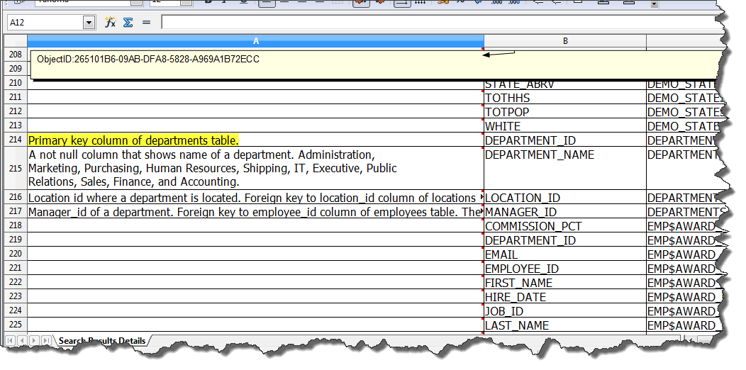
Exporting Table Column Comments to Excel using Oracle SQL Developer Data Modeler

Excel charts: how to move data labels to legend @Matt_Fischer-Daly . You can't do that, but you can show a data table below the chart instead of data labels: Click anywhere on the chart. On the Design tab of the ribbon (under Chart Tools), in the Chart Layouts group, click Add Chart Element > Data Table > With Legend Keys (or No Legend Keys if you prefer)

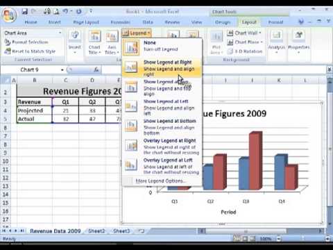
How to add or remove legends, titles or data labels in MS Excel - YouTube

Custom Data Labels with Colors and Symbols in Excel Charts - [How To ... Step 4: Select the data in column C and hit Ctrl+1 to invoke format cell dialogue box. From left click custom and have your cursor in the type field and follow these steps: Press and Hold ALT key on the keyboard and on the Numpad hit 3 and 0 keys. Let go the ALT key and you will see that upward arrow is inserted.

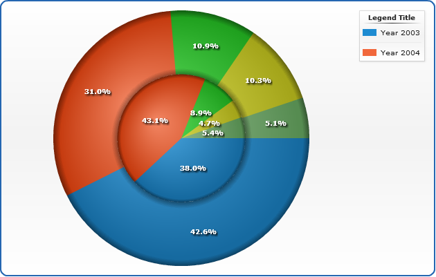
Pie and Donut Chart

How to Print Labels from Excel - Lifewire Select Mailings > Write & Insert Fields > Update Labels . Once you have the Excel spreadsheet and the Word document set up, you can merge the information and print your labels. Click Finish & Merge in the Finish group on the Mailings tab. Click Edit Individual Documents to preview how your printed labels will appear. Select All > OK .

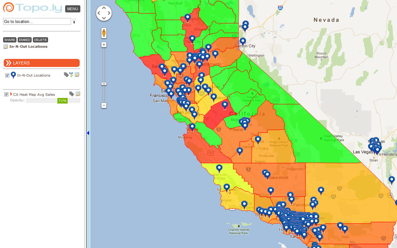
Improve Data Visualization By Mapping with Microsoft Excel | Pressat

How to add data labels from different column in an Excel chart? Click any data label to select all data labels, and then click the specified data label to select it only in the chart. 3. Go to the formula bar, type =, select the corresponding cell in the different column, and press the Enter key. See screenshot: 4. Repeat the above 2 - 3 steps to add data labels from the different column for other data points.

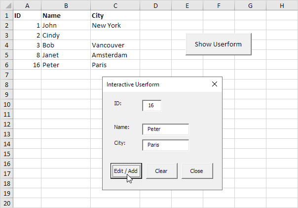
Excel VBA Interactive Userform - Easy Excel Macros

How to Print Labels From Excel - EDUCBA Navigate towards the folder where the excel file is stored in the Select Data Source pop-up window. Select the file in which the labels are stored and click Open. A new pop up box named Confirm Data Source will appear. Click on OK to let the system know that you want to use the data source. Again a pop-up window named Select Table will appear.

Display Excel data table nicely on mobile phones, without coding | by Leroy Yue | PikaPage | Medium

Excel tutorial: How to use data labels Generally, the easiest way to show data labels to use the chart elements menu. When you check the box, you'll see data labels appear in the chart. If you have more than one data series, you can select a series first, then turn on data labels for that series only. You can even select a single bar, and show just one data label.

highcharts - Optimal display for overlapping series in a line chart - Stack Overflow

How to hide zero data labels in chart in Excel? - ExtendOffice In the Format Data Labelsdialog, Click Numberin left pane, then selectCustom from the Categorylist box, and type #""into the Format Codetext box, and click Addbutton to add it to Typelist box. See screenshot: 3. Click Closebutton to close the dialog. Then you can see all zero data labels are hidden.

Share :